rollcontrol

Roll Control

Purpose: Our May 2009 launch of LV2.3 was a huge success, but our on board video could have been better if the rocket didn't spin about the longitudinal axis.

There are two ways to correct this:

Find a better way to align the fins.
Implement an active roll axis control system to stop the rotation and actively orient the rocket in the desired orientation.

Aligning the fins should be done to minimize drag on the rocket, but an active roll control system can ensure minimal roll, and even point the on board camera in an interesting direction through the launch and recovery. Further, an experiment with roll control provides a good chance to validate a control system designed based on a dynamic model.

Requirements:

Small 'canard' style fins, so that they fail safe.
On error, fins go to neutral.
Fins have short mechanical travel to minimize control gain.
Fins are mechanically linked to ensure they must operate together, only in the roll (rocket) axis.
Fins placed near CG to minimize steering if alignment is off.
One powerful/fast servo, instead of many.
If we are really worried about uC failures, we could do a hardware watchdog CPLD that centers the servo if it doesn't get serviced. That requires 1 chip and a few caps.

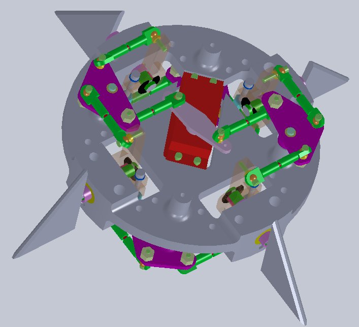
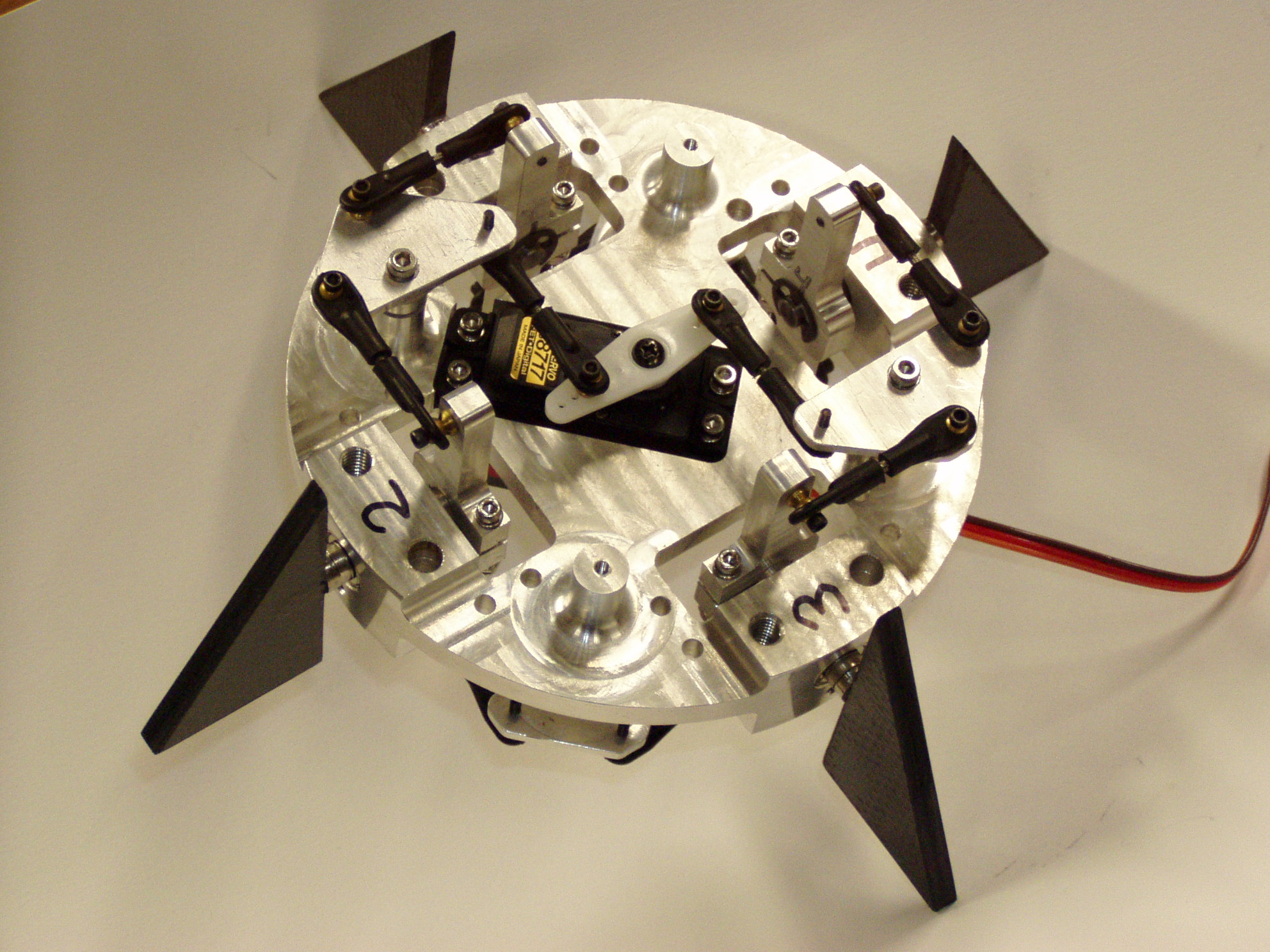
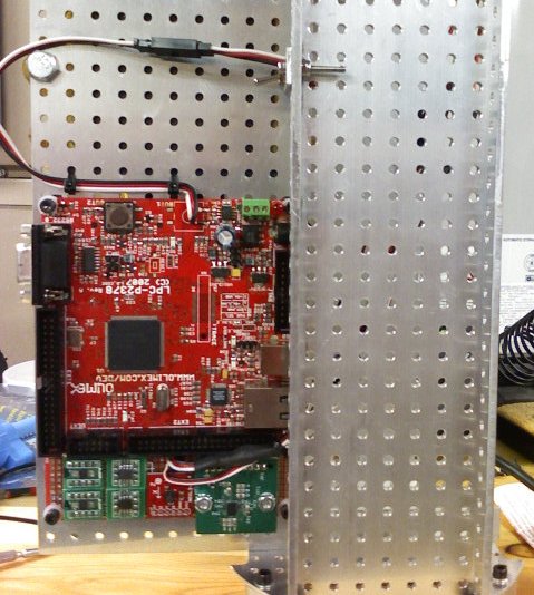
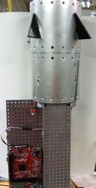
Current Design

This is a screenshot of our current design that we are going to fly. Construction complete!

Next items needed:

Fin equations relating fin length, width, airspeed, air-density, and angle-of-attack to lift and drag (done)
Post mass moment of inertia calculations (done)
Equations of motion describing the plant (done)
State-Space representation of plant (done)
Pole placement and control design (done)

Analysis

At some point, our project will require the full inertia tensor. For now however, we can achieve excellent roll control using a single degree of freedom (1 DOF) model of the rocket dynamics about the longitudinal (roll) axis.

Mass Moment of Inertia

To begin, we measure the mass moment of inertia I_zz (see CoordinateSystem) using a basic technique from any ME vibrations or physics class. Skipping the derivation, it is known that a poorly damped mass will oscillate when suspended by a spring at a frequency given by:

$f [Hz] = \frac{ \sqrt{ k / m}} { 2 \pi}$

where k is the spring stiffness and m is the mass of the suspended object.

An analogue to this equation in the rotational case:

$f [Hz] = \frac{ \sqrt{ k_t / I_{zz}}} { 2 \pi}$

Here, I_zz is the rotational inertia of the rocket about its long (z) axis, and k_t is the torsional stiffness of a rod from which our rocket is suspended. The rod is firmly clamped to the rocket at one end, and to a support structure at the other end. It is not possible to rotate the rocket about the long axis without twisting the rod.

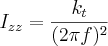
Solving the last equation for the inertia:

$I_{zz} = \frac{ k_t} { (2 \pi f)^2}$

If the rocket is rotated about the long axis (away from its resting position) and released, the inertia and the torsional spring constant will cause it to oscillate. By measuring the time it takes for the rocket to oscillate through ten cycles, the above formula can be used to calculate the rockets mass moment of inertia about the axis of oscillation.

Time Measurements

Vertical measurements were taken for the 5/31/2009 launch and for the 6/27/2010 launch:

Cycles	Time(5/31/2009) [sec]	Time(6/27/2009) [sec]
10	18.23	19.1
10	18.09	18.8
10	18.16	18.9
10	18.23	18.8
10	-	18.8

This is an average oscillation frequency of:

Launch Date	cycles/second
5/31/2009	0.5501
6/27/2009	0.5296

And for fun, we took some horizontal measurements:

19.90 seconds, 1 cycle
20.53 seconds, 1 cycle
58.81 seconds, 3 cycle

Torsion Rod

Obviously, it's necessary to select a torsion rod stiff enough to overcome drag during oscillations, yet weak enough to give oscillations that are not too fast to count. A rod that gives around 0.5 oscillations per second is about right for counting by eye and using a stopwatch. In the data above, the horizontal measurements are not useful because the wind on the rocket was easily able to overcome the torsion rod stiffness.

Our torsion rod was a 35 inch length of 1/8th inch hardened steel wire. To offset friction in the torque measuring devise, torque measurements below 3.0 inch-lbs were not used, and the angular measurement was adjusted to 0 degrees at 3.0 inch-lbs. This works well because our torque constant for the torsion rod is given by the slope of a linear regression fit applied to the torque/angle data. When twisted using a torque measuring device, the following torque/angle data was collected:

Angle [°]	Torque(rod 1) [inch · lbs]
0	3.0
10	4.8
20	6.0
25	7.0
30	7.5
45	9.0
50	10.5
60	11.75

This is an average k_t of 0.1412 [in * lbs / degree], or 0.9141 [N * m / radian] (rod 1).

Unfortunately, the torsion rod used to characterize the 5/31/09 rocket was lost/destroyed/misplaced/stolen. For the 6/27/2010 launch, a new rod assembly was constructed and characterized to have a torque constant of 0.9516 [N * m / radian] (rod 2). This is a 4% difference for a similar rod, but the rod was characterized using a different technique. When time allows, the torque constant for the new rod will be measured using similar precision to the last rod, and the numbers above will be updated.

Measured Inertia

Substituting the measured values of f and k_t to the I_zz equation, we get:

$I_{zz} = \frac{ k_t} { (2 \pi f)^2} = 0.9141 [N \cdot m] / (2 * 3.1415 * 0.5501 [Hz])^2 = 0.07652 [m^2 \cdot kg]$

This is for the 5/31/2009 rocket without the motor. Next, we'll add the engine casing to get the minimum inertia case, and then add the fuel on the pad to get the maximum inertia case.

For the rocket flown 6/27/2009, the rocket z axis inertia was:

$I_{zz} = \frac{ k_t} { (2 \pi f)^2} = 0.9516 [N \cdot m] / (2 * 3.1415 * 0.5296 [Hz])^2 = 0.08594 [m^2 \cdot kg]$

Computed Inertia

Note: The following motor and propellant mass properties are for the commercial Aerotech 98mm motor with an N2000W-P reload flown 6/27/2010. They are not representative of the experimental motor flown in the 5/31/2009 launch, which is where the above mass properties were taken.

Motor Case Inertia: To compute the inertia of the motor case, we rely on our Solidworks model. Using the density of aluminum in the model, we obtained a longitudinal axis (z-axis) mass moment of inertia of 19.05 pound * (inch^2) = 0.0055747854 m^2 kg.

Propellant Inertia: Again, using Solidworks, the propellant inertia is computed as 38.79 pounds * (inch^2) = 0.0113514922 m^2 kg.

Combined Motor Case and Propellant Inertia: The combined 'ready to fly' (complete motor) mass moment of inertia about the z-axis is computed as 57.84 pounds * (inch^2) = 0.0169262776 m^2 kg.

Canard Forces

(see the CanardAerodynamics page)

Computing canard forces relative to the canard angle-of-attack (AOA) can be a challenging problem. We have located studies, cfd analysis, and wind tunnel tests on a few interesting control fin designs. One possibly interesting step in this design might be to find a way to test the canard forces at various angles of attack near trans-sonic speeds, thereby validating our calculations and research. Short of constructing a wind tunnel, the easiest way to get 1) the speeds we want, 2) fine control of the fin AOA, and 3) accurate measurement of the fin forces produced is to attach the fin to an arm at the end of a rotating fixture, and spin the fixture at a high rotational rate. This could be accomplished by modifying a radio controlled helicopter. In place of the main rotor blades, we attach carbon fiber rods with the fins attached to the ends. Initial calculations show that we can reach fin speeds in excess of 450 MPH using a 1 meter rod spun at 3000 RPM. This is easily attainable using RC helicopter gear.

Photos Coming...

Update... It turns out that this is not so simple. Our attempt as spinning the fins using a helicopter rotor system were not completely successful. The problem was that we could not get a rotational rate higher than ~750 RPM, so the fin speeds did not exceed 150 MPH. Review of the aerodynamic properties of the rods holding the fins reveals that the drag produced by the rods is very high. In fact, the drag on the smooth, 8mm diameter round rod is ten times what it would be for an equivalent thickness airfoil. As such, the helicopter rotor system wasn't able to spin the fins fast enough.

Equations of Motion

First Principles

Equations approximating the motion of the rocket are derived from free-body diagrams (FBD) and kinetic diagrams (KD), as taught in a mid level mechanical engineering dynamics course. Developing equations in this manner is known as developing from first principles because basic Newtonian principles (f=m*a) are used to derive them. These diagrams are shown in the following figure:

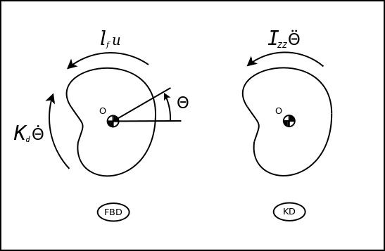
We begin our first principles analysis by summing the moments about the mass center. In the summation, we set moments in the KD on the left side of the equation, and moments in the FBD on the right side. In this analysis, positive moments are acting in the direction of positive $\theta$ :

$I_{zz} \overset{\centerdot \centerdot}{\theta} \\ = l_{f} u - k_{d} \overset{\centerdot}{\theta} \\$

State-Space

One of the (control) industry standard representations for equations of motion is the state space format. State space representations easily lend themselves to pole placement exercises and simulations. Rather than re-invent the last 100 years of control theory development, we opt to use a state-space representation:

$\left [ \begin{matrix} \overset{\centerdot \centerdot}{\theta} \\ \overset{\centerdot}{\theta} \end{matrix} \right ] = \left [ \begin{matrix} -k_{d}/I_{zz} & 0 \\ 1 & 0 \end{matrix} \right ] \left [ \begin{matrix} \overset{\centerdot}{\theta} \\ \theta \end{matrix} \right ] + \left \lbrace \begin{matrix} l_{f}/I_{zz} \\ 0 \end{matrix} \right \rbrace \cdot u$

It is assumed that all fins are acting together at the same angle of attack and in opposing directions such that they only cause rotations about the z axis. In the above equation, the sum force of the fins acting to rotate the rocket is given as , and that sum force acts at a distance $l_{f}$ from the z axis.

Model Validation

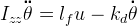
One way to validate the accuracy of our 1DOF model is by adding our torsion spring specs to the model, setting a non-zero initial value to the (angular) position state variable, and then simulating the system in time. If our model is correct, we should observe an oscillation close (in frequency) to the oscillations measured with our rocket hanging from a torsion rod. To do this, we add a $k_{t}$ term to our matrix and assign $k_{t} = 0.9141 [N \cdot m] / Radian.$

$\left [ \begin{matrix} \overset{\centerdot \centerdot}{\theta} \\ \overset{\centerdot}{\theta} \end{matrix} \right ] = \left [ \begin{matrix} -k_{d}/I_{zz} & -k_{t}/I_{zz} \\ 1 & 0 \end{matrix} \right ] \left [ \begin{matrix} \overset{\centerdot}{\theta} \\ \theta \end{matrix} \right ]$

We assign:

$k_{d} = 0.002$ (very light damping)

$k_{t} = 0.9141 [N \cdot m] / Radian.$

$I_{zz} = 0.07654 [m^2 \cdot kg]$

The result of this simulation gives a period of oscillation of 1.8182 seconds, which is very close to our actual timed measurements which averaged 1.8178 seconds.

Control System Design

Overview

The control system topology (from a control theory point of view) is fairly simple for this system. This is a single-input single-output (SISO) system, so the possible controllers are many. This control problem can be solved with standard transfer function methods, state-feedback methods, LQR, LQG, MPC, and many others. There are various advantages and disadvantages to each. Instead of weighing the merits of various control laws, we will list some of the desired features of the control and discuss some that could work for us.

Desired features:

Full Control - The main intent is to keep the rocket from spinning due to misaligned fins, but it is also desirable to have control over both the rocket roll-position and roll-rate.
Robust - The control design must accommodate modeling errors for fin characteristics, rocket state (i.e. airspeed errors), mass properties, and unexpected changes to mass properties (i.e. motor stops burning early, so inertia doesn't change as expected). Further, real world systems have limits placed on inputs or outputs. For instance, a control fin may only provide linear response through a certain angle of attack (AOA). This AOA must then be limited by the controller without compromising stability.
Expandable - It may be convenient to chose a control law that works for the SISO roll model, but is expandable to the 6DOF general control case or beyond.

Control Design Candidates

Transfer Function Methods

The majority of feedback control applications use PI, PD, or PID control methods. This is because implementation of these controllers (either mechanical, electrical, or software based) is fairly easy to understand, build, and tune. By nesting PID controllers with the roll control mechanism and state-space model, both the 'Full Control' and 'Robust' requirements were achieved. In practice, the SISO control system for roll control took less than a day to simulate and tune by hand. The result gives closed loop target roll-rate and target roll-position control for the system, even with drastic modeling errors. The 'Expandable' requirement was not met because significant additional work would be required to represent the full 6DOF model, and the cross coupling between the DOF's would make PID methods even worse.

Optimal Control Methods

Optimal control methods introduce the idea of a mathematical cost function to determine the correctness of the control design. By mathematically solving for control settings that maximize performance, an optimal controller is tuned. These include LQR and LQG controllers, among others. These provide full control and some level of expandability, but may not meet our 'Robust' requirements due to limitations on our actuators and allowed flight limits.

Model-Predictive-Control MPC

As of the time of this writing, it seems as though MPC methods meet all three of our requirements. In particular, dealing with the reality of actuator and output limitations has made the MPC controller an attractive choice. MPC is far more computationally intensive than the looped PID approach, but the algorithm used is the same regardless of the number of DOF's. This makes a more general solution that could work well if our modeling is sufficiently accurate and we have sufficient computational resources.

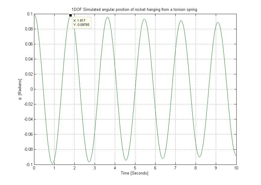
Implementation

For our June 2010 flight, the control law used for roll control will be a nested PID control. Typically, the control law would be implemented on the flight computer in floating point arithmetic. For these prototype flights, it's easier to implement the control on an LPC-2378 micro-controller (proto-board) with simple z-axis accelerometer and rate gyro sensors.

TODO list

The following is a 'laundry list' of things that need to be done with the roll control software and hardware. They are stored here, without explanation, for the purpose of tracking them to completion.

Finish launch detect tether(done)
Add stiffener braces to avionics module to control mount flex (done)
Add slow de-biasing integrator in control(skipped)
Modify derivative to reduce actuator twitch(lpf, done)
Check and remove TODO's from code base(done)
Measure flight ready mass properties (done)
- Locate torsion spring (remade, done)
Tune control for actual mass properties(done)
Bounds-test control for modeling errors in simulation(done)
Add CAN based data logging... Dual rate prelaunch/postlaunch(done)

Results

To date (11-1-2010), two flights have been equipped with roll axis stabilization. The first one, on June 27, 2010 was not successful because we neglected the aerodynamic interaction between the canards and the fins. After some research, we came to understand the aerodynamics better and corrected the problem by de-coupling the main fins in the roll axis. By attaching the fin canister to a large bearing (spin-can), the second flight on Oct 17, 2010 was a success.

The following plot shows the sensor data recorded from the Oct 17, 2010 flight:

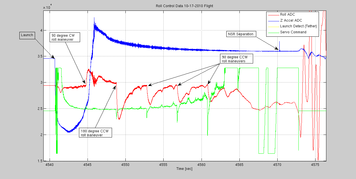
The key takeaway from this exercise was the process of modeling a dynamic system, simulating the system, and, in the simulation, tuning the control until the desired performance is achieved.

As an additional step, the inputs to the controller (launch tether status, gyro, and acceleration ADC values) were recorded together with servo commands (PWM signal sent to servo). After the flight, the recorded input signals were fed into the controller simulation, and the recorded servo commands were compared with the simulation output. The results, below, are nearly identical over the entire flight.

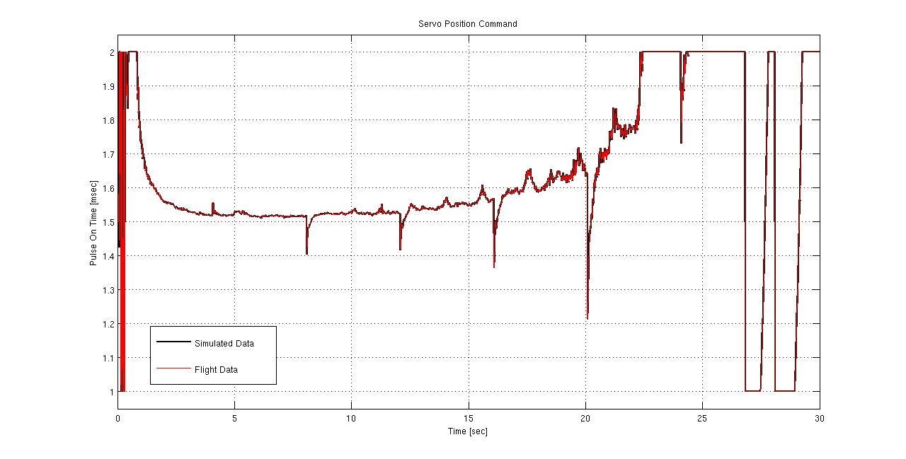
The final step in this process will be to improve our models by comparing rocket flight data response to stimulus (servo movement) with the simulation response to the same stimulus. From this comparison, we can further improve our model fidelity, and thus improve our control system.

Improvements

One mistake made in the control law was in the roll rate PID loop. A saturation limit was added to the integrator, with a limit value of 0.1 Newton * meters (0.88 inch*lbs). This was not noticed until after the flight because the simulation model did not contain a torque bias. Such a torque bias during the flight was likely caused by friction in the rotating spin can bearings. This error shows itself as sluggish response and a slight position overrun during roll maneuvers. A better limit for this integrator might be around 1.5 Newton * meters.

References

[1] Wang, Liuping PhD Model Predictive Control System Design and Implementation Using MATLAB. London: Springer-Verlag London Limited, 2009.
ISBN 978-1-84882-330-3