Staging

Stacking rockets atop one another will allow us to discard fuel tanks and motors en route to orbit, reducing the amount of mass we need to accelerate in a stepwise manner.

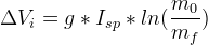
The modified rocket equation for staging is:

${\Delta}V_i = g*I_{sp}*ln(\frac{m_0}{m_f})$ (S-1)

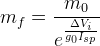
Which expands neatly to the mass-calculating functions:

$\frac{m_0}{m_f} = e^\frac{{\Delta}V_i}{g_0I_{sp}}$ (S-2.a) $m_f = \frac{m_0}{e^\frac{{\Delta}V_i}{g_0I_{sp}}}$ (S-2.b) $m_0 = m_f*e^\frac{{\Delta}V_i}{gI_{sp}}$ (S-2.c)

The Braeunig site suggests that: 1. Isp's should decrease from the top stage. 2. Higher Isp's should correspond to higher delta-v's on a stage-by-stage examination. 3. Each stage should be smaller than the one below it. 4. Similar stages should provide the same delta-v.

Our requirements:

Bear skins and stone knives (knapped flint is okay).
Bigger = more complex. Inverse relationship between degree of complexity and PSAS' comfort with a given solution.
Control authority along entire trajectory to orbit. Extreme reluctance to relinquish authority.
Further calculations to find:

Considerations developed from requirements:

The Roll Control module can be modified/scaled for control authority in atmosphere. Given requirement 2, this suggests (in conjunction with Braeunig guideline 1 for staging) that we use solid boosters for the first stage, as they are simple and control authority will derive from actuated fins.
Second stage will likely require vectored thrust, and will if we choose a 2-stage rocket.
- Propulsion team members have proposed a bimodal second stage with a main, unvectored motor and two supplemental, vectoring thrusters.
Further calculations to define:
1. Final delta-v (9100 m/s expected).
2. Payload mass (1kg expected).
3. Dead weight for each stage.

Topics for Further Inquiry

At what height do we expect the launch platform to drop the first stage?
At what height do we expect the launch platform to begin insertion maneuvers?
Does anyone know anything about optimal orbital insertion trajectories? A brief Googling reveals that genetic algorithms might be of interest.
What are the advantages and disadvantages of adding a third stage for insertion?

An Iterative Approach to Staging Design

We consider in this example a 3 stage rocket with stages 1,2,3 numbered from top to bottom. In accordance with our BSSK approach, we consider each stage to have a solid booster with Isp of 250.

The question might arise: how much fuel would be required to get a 1kg payload into orbit around the earth?

An obvious point of departure is the delta-v required to achieve low Earth orbit. Previous PSAS research has shown this to be ~9100 m/s (https://archive.psas.pdx.edu/news/2000-11-02/sld003/).

We describe here a method for estimating fuel and dead weights iteratively. Find the amount of fuel required to provide the desired change in velocity. Estimate the amount of weight required on-rocket in infrastructure to support, feed, combust and exhaust that amount of fuel. Add the infrastructure weight to the original payload weight and recalculate the amount of fuel necessary to provide the desired change in velocity.

These two files are designed to take values for stage numbers and data about each stage and compute the other design parameters. Values are stored in staging2inputs.m and running that calls staging2.m.

From the iterator, starting with a 1 kg payload and conservative Isp/mass fraction values:

Attribute	Stage 1	Stage 2	Stage 3
delta-V (m/s)	3033.3	3033.3	3033.3
Isp (s)	250	250	250
Mass Fraction	.8	.8	.8
Payload Mass (kg)	1	6.74	45.43
Burnout Mass (kg)	1.9567	13.188	88.72
Ignition mass (kg)	6.74	45.428	306.1843

Maneuver Burn Time

In designing rocket motors, we are interested in how long a combustion chamber and De Laval nozzle assembly are required to perform in service. This is given off the Braeunig site as:

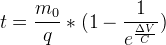$t = \frac{m_0}{q}*(1-\frac{1}{e^\frac{{\Delta}V}{C}})$ (S-4) where $C = I_{sp}*g_0$

Thrust as a Function of Loading from Acceleration

From Newtonian physics, we know that F = m*a .

We can rearrange this to show the acceleration that a rocket experiences as a function of specific impulse, mass flow rate and initial or final masses (assume for the purpose of stone-knife and bearskin engineering that thrust magnitude is not variable):

$a_0 = \frac{I_{sp}g_0q}{m_0}$ (S-5.a) $a_f = \frac{I_{sp}g_0q}{m_f}$ (S-5.b)

The Iterator takes the quotient of a0 and af with 9.81 to find the acceleration load in terms of earth-normal gravities. It is required to provide a mass-flow rate from the nozzle to determine this value.

We can rearrange S-5 to show mass flow as a function of acceleration as expressed in gravities:

$a = \frac{I_{sp}g_0q}{m} {\Rightarrow} q = \frac{am_0}{I_{sp}g_0} {\Rightarrow} q = \frac{ng_0m}{I_{sp}{g_0}} {\Rightarrow} q = \frac{nm}{I_{sp}}$