Basics
Example
Derivation

Basics

Given a system model, an initial system state, and a sequence of noisy measurements, a Kalman filter can be constructed to produce a sequence of state estimates that are optimal in the sense that they minimize the expected square-error between the estimates and the true system state.

Summary of Kalman Filter Symbols

Symbol	Definition	Name
x	n×1	system state vector
Φ (Phi)	n×n	state transition matrix
P	n×n	state error covariance matrix
u	u×1	control input vector
Γ (Gamma)	n×u	control input Matrix
w	q×1	process noise vector
Λ (Lambda)	n×q	process noise input matrix
Q	q×q	process noise covariance matrix
y	m×1	output vector
H	m×n	output matrix
ν (nu)	m×1	measurement noise vector
R	m×m	measurement noise covariance matrix
K	n×m	Kalman gain, feedback matrix

Table (1)

Typical Kalman Filter Equations

Equation	Description
$\bf{\hat x_0} = \it E[\bf{x_0}]$	state initialization
$\bf{P_0} = \it E[(\bf{\hat x_0 - x_0})^2]$	state error initialization
$\bf{x_k^-} = \bf{\Phi_{k-1} \hat x_{k-1} + \Gamma_{k-1} u_{k-1}}$	state propagation Previous knowledge of the system is used to guess the future state.
$\bf{P_k^-} = \bf{\Phi_{k-1} P_{k-1} \Phi_{k-1}^{\rm T} + \Lambda_{k-1} Q_{k-1} \Lambda_{k-1}^{\rm T}}$	state error propagation System dynamics effect the error. Process noise increases the error.
$\bf{K_k} = \bf{P_k^-\, H_k^{\rm T} (H_k P_k^-\, H_k^{\rm T} + R_k)^{-1}}$	Kalman gain update Recursive least squares solution, trades off state uncertainty and measurement noise.
$\bf{\hat x_k} = \bf{x_k^- + K_k (\tilde y_k - H_k x_k^-)}$	measurement update New optimal state estimate
$\bf{P_k} = \bf{((P_k^-)^{-1} + H_k^{\rm T} R_k^{-1} H_k)^{-1}}$	state error update new measurements add to knowledge of system, estimated error decreases

Table (2)

Start with the discreet linear dynamic system equation

$\displaystyle (1.1)\quad\ \bf{x_{k+1}} = \bf{\Phi_k\ x_k} + \bf{\Gamma_k} \bf{u_k} + \bf{\Lambda_k} \bf{w_k}$

And the measurement equation

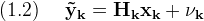
$\displaystyle (1.2)\quad\ \bf{\tilde y_k} = \bf{H_k} \bf{x_k} + \bf{\nu_k}$

Where the subscript (·_k) indicates the value at time step (t_k)

Although the form of the system equations would seem to apply only to strictly linear systems, as usual, various linearizations and quasi-non-linear techniques can be applied to extend the Kalman filter to a variety of real world non-linear problems.

Making some key assumptions will greatly simplify what follows.
Assume that

For each time step (k); (Φ_k), (Γ_k), (Λ_k), (H_k) and (u_k) are known without error
Noise components (w_k) and (ν_k) are uncorrelated Gaussian random sequences with zero mean
The noise covariance matrices are known, (cov[w_k]=Q_k), (cov[ν_k]=R_k)

In principle these assumptions can be relaxed somewhat. For example, if any of the system matrices contain random components, those components may be factored out into the noise vectors. Similarly, any noise process that is representable as a linear combination of white Gaussian noise can be modeled by adding extra states to the system and driving those extra states with zero mean Gaussian noise. Even if the noise matrices are not known exactly, they can be estimated, or calculated on line, or discovered by system tuning.

The exact quantity minimized by a Kalman filter is the matrix (P), the state error covariance matrix

$\displaystyle (1.3)\quad\ \bf{P} \equiv \it{E}[\bf{(\hat x-x)}^2]$

Where (E ) is a function returning the expectation of a random variable

The estimated state (x̂) that minimizes (P) is found by solving a weighted least squares problem. The weights for the computation ultimately come from the process noise covariance matrix (Q) and the measurement noise covariance matrix (R). The actual output of the filter is a sequence of linear combinations formed from the predicted state (x⁻), and the current measurements of the system (ỹ). Technically these outputs are known as the best linear unbiased estimates. The existence of such estimates is guaranteed only with certain restrictions, see the section on complications. (FIXME: complications section not built yet)

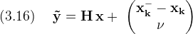
Typically the Kalman filter is implemented recursively as a predictor-corrector system. In the prediction step, knowledge of the past state of the system is used to extrapolate to the system's state at the next time step. Once the next time step is actually reached and new measurements become available, the new measurements are used to refine the filter's estimate of the true state like this

$\displaystyle (1.4)\quad\ \bf{\hat x_k} = \bf{x_k^-} + \bf{K_k}(\bf{\tilde y_k}-\bf{H_k}\bf{x_k^-})$

Where the matrix (K_k), the Kalman gain, or feedback matrix, is chosen so that (P_k) is minimized

Later there will be some justification, but for now accept that one possible choice for (K_k) is

$\displaystyle (1.5)\quad\ \bf{K_k} = \bf{P_k^-\, H_k^{\rm T} (H_k P_k^-\, H_k^{\rm T} + R_k)^{-1}} = \bf{\frac {P_k^-\, H_k^{\rm T}}{H_k P_k^-\, H_k^{\rm T} + R_k}}$

Where the measurement noise covariance matrix (R_k) is defined as

$\displaystyle (1.6)\quad\ \bf{R} \equiv \mbox{\rm cov}[\bf{\nu}] = \it E[\bf{\nu}^2]$

The relative magnitudes of matrices (R_k) and (P_k) control a trade-off between the filter's use of predicted state estimate (x_k⁻) and measurement (ỹ_k).

Consider some limits on (K_k)

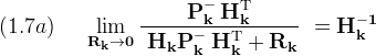
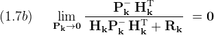
$\displaystyle (1.7a)\quad\ \lim\limits_{\bf{R_k \to 0}} \bf{{P_k^-\, H_k^{\rm T}} \over\ {H_k P_k^-\, H_k^{\rm T} + R_k}}\ = \bf{H_k^{-1}}$

$\displaystyle (1.7b)\quad\ \lim\limits_{\bf{P_k \to 0}} \bf{{P_k^-\, H_k^{\rm T}} \over\ {H_k P_k^-\, H_k^{\rm T} + R_k}}\ = \bf 0$

Substituting the first limit into the measurement update equation (1.4) suggests that when the magnitude of (R) is small, meaning that the measurements are accurate, the state estimate depends mostly on the measurements. Likewise when the state is known accurately, then (H P⁻ H^T) is small compared to (R), and the filter mostly ignores the measurements relying instead on the prediction derived from the previous state (x_k⁻).

Example

Simple Kalman Example

Derivation

The desired Kalman filter implementation is linear and recursive, that is, given the old filter state (𝓕_k-1) and new measurements (𝓜_k) the new filter state is calculated as

$\displaystyle (3.1a)\quad\ {\cal F}_k^- = \it g [{\cal F}_{k-1}]$

$\displaystyle (3.1b)\quad\ {\cal F}_k = \it f [{\cal F}_k^-\,,\ {\cal M}_k]$

Where ( f and g ) are linear functions

Referring to table(2), the sequence of equations shown are both linear and recursive as desired. Though so far, little explanation has been given to justify their use. In order to maintain some credibility, and to prove we aren't total mathematical wimps, we will attempt a derivation of these equations. The goal here is not mathematical perfection, rather clarity without serious error.

Fundamentally Kalman filtering involves solving a least squares error problem. Specifically, given a state estimate (x⁻) of known covariance (P⁻) and a new set of measurements (ỹ) with covariance (R), find a new state estimate (x̂) such that the new state error covariance (P) is minimized.

For the predicted state error write

$\displaystyle (3.2)\quad\ \bf \mbox{\rm cov}[\bf{x^- - x}] = \bf P^-$

Likewise for the measurement error

$\displaystyle (3.3)\quad\ \bf \mbox{\rm cov}[\bf{\tilde y - y}] = \bf R$

Seek a new state vector (x̂) such that the (n+m×1) combined state error vector

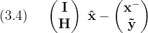
$\displaystyle (3.4)\quad\ \begin{pmatrix} \bf I \\ \bf H \end{pmatrix}\ \bf{\hat x} - \begin{pmatrix} \bf x^- \\ \bf{\tilde y} \end{pmatrix}$

Is minimized in the weighted least squares sense

The chief difficulty with Kalman filter theory is contained in (3.4). The errors in (3.2) and (3.3) are defined in terms of the true state and exact measurements, but while operating the filter, all that is available are estimates and noisy measurements. In equation (3.4) the measurement (ỹ) and the estimated state (x⁻) have been used where the exact values would seem to be appropriate. Here's a simple-minded explanation of why it's ok to use the imprecise values in (3.4): The noise has been assumed to be zero-mean, therefore the expectation of the approximate values are the correct true values, so using the approximate values will produce unbiased estimates. Further, since it has been assumed that the covariance of both (ỹ) and (x⁻) are known, the weighted least squares process has enough information to properly minimize the total square error.

Whether the previous paragraph constitutes a satisfactory justification of (3.4) is a question worth pondering. If not there are many, many, many, books that address this issue (try looking up stochastic least squares). (However the chances of finding a very clear explanation appear to be low.) The issue is significant in as much as once (3.4) is accepted, Kalman filtering as a theoretical matter is essentially solved. Though, solved in this sense is still far from a practical implementation. To derive a practical filter, some clever arithmetic is required.

A weighted least squares solution minimizes a scalar cost function (𝓙), here written in matrix form

$\displaystyle (3.5)\quad\ \cal{J}[\bf \epsilon , \bf W] = \bf{\epsilon}^{\rm T} \, \bf W \, \bf \epsilon$

Where the matrix (W) is the weighting for the cost function. The weighting can be any positive definite matrix.

In formulating the Kalman filter the noise statistics have been defined in terms of covariance, and since elements with large covariance should be given low weight, the correct weighting matrix for this problem is the inverse of the covariance matrix. This is appealing intuitively and not too difficult to prove, though no proof is given here.

Using the inverse covariance as the weighting function and referring to (3.4) the cost function for the Kalman filter is

$\displaystyle (3.6)\quad\ \cal{J} =\ \begin{pmatrix}\ \bf{I\, \hat x_k} - \bf{x_k^-} \\\ \bf{H_k \hat x_k} - \bf{\tilde y_k}\ \end{pmatrix}^{\rm T}\ \begin{pmatrix}\ \bf P_k^- & \bf 0 \\ \bf 0 & \bf R_k\ \end{pmatrix}^{\rm -1}\ \begin{pmatrix}\ \bf{I \, \hat x_k} - \bf{x_k^-} \\ \bf{H_k \hat x_k} - \bf{\tilde y_k} \end{pmatrix}$

Where the block matrices shown have dimensions (n+m×1) and (n+m×n+m) respectively

The notational mapping suggested by (3.4) is

$\displaystyle (3.7)\quad\ \left\{\ \begin{pmatrix} \bf I \\ \bf H_k \end{pmatrix}\ \rightarrow \bf H,\ \bf{\hat x_k} \rightarrow \bf{\hat x},\ \begin{pmatrix} \bf x_k^- \\ \bf{\tilde y_k} \end{pmatrix}\ \rightarrow \bf{\tilde y},\ \begin{pmatrix} \bf P_k^- & 0 \\ 0 & \bf R_k \end{pmatrix} \rightarrow \bf{R}\ \right\}$

Use this mapping to state the cost function in a slightly more generic form as

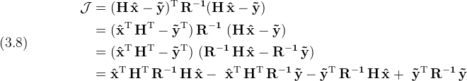
$\displaystyle (3.8)\quad\ \begin{split} \cal{J}& = \bf{(H\,\hat x - \tilde y)^{\rm T}\,R^{-1} (H\,\hat x - \tilde y})\\ & = (\bf{\hat x^{\rm T} \, H^{\rm T} - \tilde y^{\rm T}})\,\bf R^{-1}\ (\bf{H\,\hat x - \tilde y})\\ & = (\bf{\hat x^{\rm T}\,H^{\rm T} - \tilde y^{\rm T}})\ (\bf{R^{-1}\,H\,\hat x - R^{-1}\,\tilde y})\\ & = \bf{\hat x^{\rm T}\,H^{\rm T}\,R^{-1}\,H\,\hat x -\ \hat x^{\rm T}\,H^{\rm T}\,R^{-1}\,\tilde y - \tilde y^{\rm T}\,R^{-1}\,H\,\hat x +\ \tilde y^{\rm T}\,R^{-1}\,\tilde y} \end{split}$

In (3.8) the cost function has been expanded in anticipation of taking derivatives. (A matrix derivative typically involves taking a transpose.)

Returning to the generic minimization problem, take the partial derivative

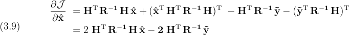
$\displaystyle (3.9)\quad\ \begin{split}\ \frac{\partial\cal{J}} {\partial\bf{\hat x}}\ & = \bf{H^{\rm T}\,R^{-1}\,H\,\hat x + (\hat x^{\rm T}\,H^{\rm T}\,R^{-1}\,H)^{\rm T}\ - H^{\rm T}\,R^{-1}\,\tilde y - (\tilde y^{\rm T}\,R^{-1}\,H)^{\rm T}}\\\ & = 2\ \bf{H^{\rm T}\,R^{-1}\,H\,\hat x} - 2\ \bf{H^{\rm T}\,R^{-1}\,\tilde y}\\\ \end{split}$

Set the derivative to zero and solve for (x̂)

$\displaystyle (3.10)\quad\ \bf{\hat x} = \bf{(H^{\rm T}\,R^{-1}\,H)^{-1}\,H^{\rm T}\,R^{-1}\,\tilde y}$

This is the classic weighted least squares solution.

Applying (3.10) to our original problem using (3.7) gets

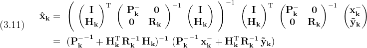
$\displaystyle (3.11)\quad\ \begin{split}\ \bf{\hat x_k} & =\ \left(\ \begin{pmatrix} \bf I \\ \bf H_k \end{pmatrix}^{\rm T}\ \begin{pmatrix}\ \bf P_k^- & \bf 0 \\ \bf 0 & \bf R_k\ \end{pmatrix}^{-1}\ \begin{pmatrix} \bf I \\ \bf H_k \end{pmatrix}\ \right)^{-1}\ \begin{pmatrix} \bf I \\ \bf H_k \end{pmatrix}^{\rm T}\ \begin{pmatrix} \bf P_k^- & \bf 0 \\ \bf 0 & \bf R_k \end{pmatrix}^{-1}\ \begin{pmatrix} \bf x_k^- \\ \bf{\tilde y_k} \end{pmatrix}\\\ & =\ (\bf{P_k^-}^{-1}+\bf{H_k^{\rm T}\, R_k^{-1}\,H_k})^{-1}\ (\bf{P_k^-}^{-1}\,\bf{x_k^- + H_k^{\rm T}\, R_k^{-1}\,\tilde y_k})\ \end{split}$

There's nothing wrong with the form given in (3.11), but for various reasons it's desirable to exhibit the measurement update form (1.4). To do this everyone uses the matrix inversion lemma

$\displaystyle (3.12)\quad\ \bf{(A-B^{\rm T}\,C^{-1}\,B)^{-1} =\ A^{-1}-A^{-1}\,B^{\rm T}(B\,A^{-1}B^{\rm T}-C)^{-1}B\,A^{-1}}$

Using the mapping

$\displaystyle (3.13)\quad\ \left\{ \bf A \rightarrow \bf{P_k^-}^{-1},\ \ \bf B \rightarrow \bf H_k ,\ \ \bf C \rightarrow -\bf R_k \ \ \right\}$

The solution given by (3.11) becomes

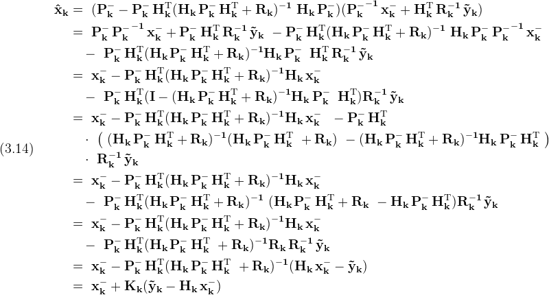
$\displaystyle (3.14)\quad\ \begin{split}\ \bf{\hat x_k} & = \bf{\ (P_k^- - P_k^-\,H_k^{\rm T} (H_k\,P_k^-\,H_k^{\rm T} + R_k)^{-1}\ H_k\,P_k^-) ({P_k^-}^{-1}\,x_k^- + H_k^{\rm T}\,R_k^{-1}\,\tilde y_k) }\\\ & = \bf{\ P_k^-\,{P_k^-}^{-1}\,x_k^- + P_k^-\,H_k^{\rm T}\,R_k^{-1}\,\tilde y_k\ - P_k^-\,H_k^{\rm T}(H_k\,P_k^-\,H_k^{\rm T} + R_k)^{-1}\ H_k\,P_k^-\,{P_k^-}^{-1}\,x_k^-}\\\ &\quad - \bf{\ P_k^-\,H_k^{\rm T}(H_k\,P_k^-\,H_k^{\rm T} + R_k)^{-1}H_k\,P_k^-\,\ H_k^{\rm T}\,R_k^{-1}\,\tilde y_k}\\\ & = \bf{\ x_k^- - P_k^-\,H_k^{\rm T}(H_k\,P_k^-\,H_k^{\rm T} + R_k)^{-1}H_k\,x_k^-}\\\ &\quad - \bf{\ P_k^-\,H_k^{\rm T}(I-(H_k\,P_k^-\,H_k^{\rm T} + R_k)^{-1}H_k\,P_k^-\,\ H_k^{\rm T})R_k^{-1}\,\tilde y_k}\\\ & = \bf{\ x_k^- - P_k^-\,H_k^{\rm T}(H_k\,P_k^-\,H_k^{\rm T} + R_k)^{-1}H_k\,x_k^-\ \ - P_k^-\,H_k^{\rm T}}\\\ &\quad \cdot \bf{\ \left(\ (H_k\,P_k^-\,H_k^{\rm T} + R_k)^{-1}(H_k\,P_k^-\,H_k^{\rm T}\ + R_k)\ - (H_k\,P_k^-\,H_k^{\rm T} + R_k)^{-1}H_k\,P_k^-\,H_k^{\rm T}\ \right)}\\\ &\quad \cdot \bf{\ R_k^{-1}\,\tilde y_k}\\\ & = \bf{\ x_k^- - P_k^-\,H_k^{\rm T}(H_k\,P_k^-\,H_k^{\rm T} + R_k)^{-1}H_k\,x_k^-}\\\ &\quad - \bf{\ P_k^-\,H_k^{\rm T}(H_k\,P_k^-\,H_k^{\rm T} + R_k)^{-1}\ (H_k\,P_k^-\,H_k^{\rm T} + R_k\ - H_k\,P_k^-\,H_k^{\rm T})R_k^{-1}\,\tilde y_k}\\\ & = \bf{\ x_k^- - P_k^-\,H_k^{\rm T}(H_k\,P_k^-\,H_k^{\rm T} + R_k)^{-1}H_k\,x_k^-}\\\ &\quad - \bf{\ P_k^-\,H_k^{\rm T}(H_k\,P_k^-\,H_k^{\rm T}\ + R_k)^{-1}R_k\,R_k^{-1}\,\tilde y_k}\\\ & = \bf{\ x_k^- - P_k^-\,H_k^{\rm T}(H_k\,P_k^-\,H_k^{\rm T}\ + R_k)^{-1}(H_k\,x_k^- - \tilde y_k) }\\\ & = \bf{\ x_k^- + K_k (\tilde y_k - H_k\,x_k^-) } \end{split}$

Which matches the measurement update form given in (1.4) with (K_k) as in (1.5)

It's possible to derive the state error update equation directly from the definition given in (1.3) and repeated here

$\displaystyle (3.15)\quad\ \bf{P} \equiv \it{E}[\bf{(\hat x - x)}^2]$

It would be very convenient to write the true state (x_k) in terms of (x̂), in fact the previous hand-waving argument in support of equation (3.4) implies this must be possible.

Using the mapping defined in (3.7), the measurement equation is

$\displaystyle (3.16)\quad\ \bf{\tilde y = H\,x +\ \begin{pmatrix} \bf{x_k^- - x_k} \\ \bf \nu \end{pmatrix}}$

According to our least squares solution (3.10)

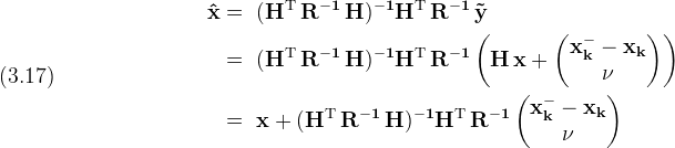
$\displaystyle (3.17)\quad\ \begin{split}\ \bf{\hat x} & =\ \bf{(H^{\rm T}\,R^{-1}\,H)^{-1} H^{\rm T}\,R^{-1}\,\tilde y}\\\ & =\ \bf{(H^{\rm T}\,R^{-1}\,H)^{-1}H^{\rm T}\,R^{-1}} \left( \bf{H\,x + \begin{pmatrix} \bf{x_k^- - x_k} \\ \bf \nu \end{pmatrix}} \right)\\\ & =\ \bf{x + (H^{\rm T}\,R^{-1}\,H)^{-1} H^{\rm T}\,R^{-1} \begin{pmatrix} \bf{x_k^- - x_k} \\ \bf \nu \end{pmatrix}}\ \end{split}$

Putting this into the definition for (P)

$\displaystyle (3.18)\quad\ \begin{split}\ \bf P & =\ \it{E}[(\bf{\hat x - x})^2]\ = \it{E} \left[ \left(\ \bf{(H^{\rm T}\,R^{-1}\,H)^{-1} H^{\rm T}\,R^{-1}\ \begin{pmatrix} \bf{x_k^- - x_k} \\ \bf \nu \end{pmatrix}\ }\right)^2 \right]\\\ & = \bf{\ \left( \bf{(H^{\rm T}\,R^{-1}\,H)^{-1}H^{\rm T}\,R^{-1}} \right)\ \it{E} \left[\ \begin{pmatrix} \bf{x_k^- - x_k} \\ \bf{\nu} \end{pmatrix}^2\ \right]\ \left(\ \bf{(H^{\rm T}\,R^{-1}\,H)^{-1}H^{\rm T}\,R^{-1}}\ \right)^{\rm T}}\\\ & = \bf{\ \left( (H^{\rm T}\,R^{-1}\,H)^{-1}H^{\rm T}\,R^{-1} \right)\ \,R\,\ \left( (H^{\rm T}\,R^{-1}\,H)^{-1}H^{\rm T}\,R^{-1} \right)^{\rm T}}\\\ & =\ (\bf{H^{\rm T}\,R^{-1} H})^{-1}\ \end{split}$

Substituting back the values for (H) and (R) from (3.7)

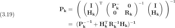
$\displaystyle (3.19)\quad\ \begin{split}\ \bf{P_k} & =\ \left(\ \begin{pmatrix} \bf I \\ \bf H_k \end{pmatrix}^{\rm T}\ \begin{pmatrix}\ \bf P_k^- & \bf 0 \\ \bf 0 & \bf R_k\ \end{pmatrix}^{-1}\ \begin{pmatrix} \bf I \\ \bf H_k \end{pmatrix}\ \right)^{-1}\\\ & =\ (\bf{{P_k^-}^{-1} + H_k^{\rm T}\,R_k^{-1} H_k})^{-1}\ \end{split}$

Equation (3.19) performs the "measurement update" for the state error estimate (P).
It can be written as a parallel sum

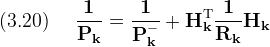
$\displaystyle (3.20)\quad\ \bf{ {1 \over P_k} = {1 \over P_k^-} + H_k^{\rm T} {1 \over R_k} H_k }$

The last term in (3.20) can be considered to represent the extra information added to the state because of the current measurement.

The form of (3.20) makes sense because adding new information (positive (R_k^-1)) will tend to decrease the system uncertainty.

Now all that remains is to derive the state error propagation equation. Again using definition (1.3)

$\displaystyle (3.21)\quad\ \bf P_{k+1}^- =\ \it{E} [ ( \bf{ x_{k+1}^- - x_{k+1} } )^2 ]$

Applying the state propagation equation (1.1) to the inside of (3.21), the control input, being common, cancels out

$\displaystyle (3.22)\quad\ ( \bf{ x_{k+1}^- - x_{k+1} } ) =\ \bf{ \Phi_k (\hat x_k - x_k) + \Gamma_k (u_k - u_k) + \Lambda_k\,w_k) }$

$\displaystyle (3.23)\quad\ \bf{P_{k+1}^-} = \it{E}[ \bf{ \Phi_k (\hat x_k - x_k)^2 \Phi_k^{\rm T} +\ \Lambda_k\,w_k^2\,\Lambda_k^{\rm T} + \Phi_k (\hat x_k - x_k) w_k^2\,\Lambda_k^{\rm T} + \Lambda_k\,w_k (\hat x_k - x_k)^2 \Phi_k^{\rm T} } ]$

In (3.23) the expectation of the cross terms is zero because (x_k) contains terms of (w_k-1) only, and by the assumption that (w) is white noise.

$\displaystyle (3.24)\quad\ \it{E}[ \bf{ w_k\,w_{k-1} } ] = \bf 0$

So finally

$\displaystyle (3.25)\quad\ \bf{P_{k+1}^-} = \bf{ \Phi_k\,P_k\,\Phi_k^{\rm T} + \Lambda_k\,Q_k\,\Lambda_k^{\rm T} }$

The derivation of the equations in table(2) is now complete.